Building an Image Search Engine: Defining Your Image Descriptor (Step 1 of 4)
During that blog post, I made mention to the four steps of building an image search engine:
- Defining your descriptor: What type of descriptor are you going to use? What aspect of the image are you describing?
- Indexing your dataset: Apply your descriptor to each image in your dataset.
- Defining your similarity metric: How are you going to determine how “similar” two images are?
- Searching: How does the actual search take place? How are queries submitted to your image search engine?
Defining Your Image Descriptor
In our Lord of the Rings image search engine, we used a 3D color histogram to characterize the color of each image. This OpenCV image descriptor was a global image descriptor and applied to the entier image. The 3D color histogram was a good choice for our dataset. The five scenes we utilized from the movies each had relatively different color distributions, thus making it easier for a color histogram to return relevant results.
Of course, color histograms are not the only image descriptor we can use. We can also utilize methods to describe both the texture and shape of objects in an image.
Let’s take a look:
Color
As we’ve already seen, color is the most basic aspect of an image to describe, and arguably the most computationally simple. We can characterize the color of an image using the mean, standard deviation, and skew of each channel’s pixel intensities. We could also use color histograms as we’ve seen in other blog posts. In color histograms are global image descriptors applied to the entire image.
One benefit of using simple color methods is that we can easily obtain image size (scale) and orientation (how the image is rotated) invariance.
How is this possible?
Well, let’s take a look at this model of Jurassic Park’s T-Rex at varying scales and orientations, and the resulting histograms extracted from each image.
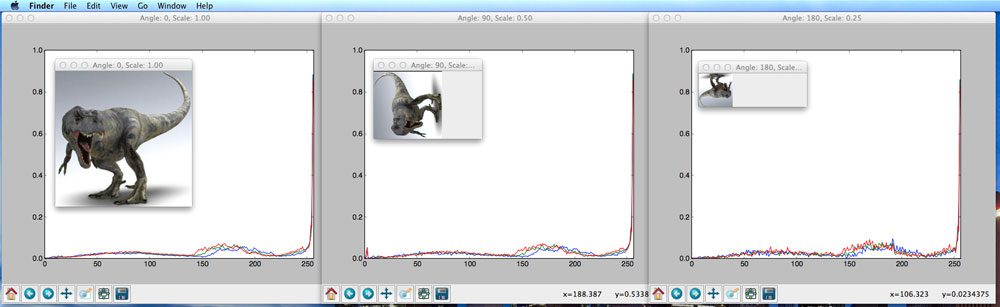
Figure 1: No matter how we rotate and scale the T-Rex image, we still have the same histogram.
As you can see, we rotate and resize the image with a varying number of angles and scaling factors. The number of bins is plotted along the X-axis and the percentage of pixels placed in each bin on the Y-axis.
In each case, the histogram is identical, thus demonstrating that the color histogram does not change as the image is scaled and rotated.
Rotation and scale invariance of an image descriptor are both desirable properties of an image search engine. If a user submits a query image to our image search engine, the system should find similar images, regardless of how the query image is resized or rotated. When a descriptor is robust to changes such as rotation and scale, we call them invariants due to the fact that the descriptor is invariant (i.e. does not change) even as the image is rotated and scaled.
Texture
Texture tries to model feel, appearance, and the overall tactile quality of an object in an image; however, texture tends to be difficult to represent. For example, how do we construct an image descriptor that can describe the scales of a T-Rex as “rough” or “coarse”?
Most methods trying to model texture examine the grayscale image, rather than the color image. If we use a grayscale image, we simply have a NxN matrix of pixel intensities. We can examine pairs of these pixels and then construct a distribution of how often such pairs occur within X pixels of each other. This type of distribution is called a Gray-Level Co-occurrence Matrix (GLCM).
Once we have the GLCM, we can compute statistics, such as contrast, correlation, and entropy to name a few.
Other texture descriptors exist as well, including taking the Fourier or Wavelet transformation of the grayscale image and examining the coefficients after the transformation.
Finally, one of the more popular texture descriptors of late, Histogram of Oriented Gradients, has been extremely useful in the detection of people in images.
Shape
When discussing shape, I am not talking about the shape (dimensions, in terms of width and height) of the NumPy array that an image is represented as. Instead, I’m talking about the shape of a particular object in an image.
When using a shape descriptor, or first step is normally to apply a segmentation or edge detection technique, allowing us to focus strictly on the contour of the shape we want to describe. Then, once we have the contour, we can again compute statistical moments to represent the shape.
Let’s look at an example using this Pikachu image:

Figure 2: The image on the left is not suited for shape description. We first need to either perform edge detection (middle) or examine the countered, masked region (right).
On the left, we have the full color image of Pikachu. Typically, we would not use this type of image to describe shape. Instead, we would convert the image to grayscale and perform edge detection (center) or utilize the mask of Pikachu (i.e. the relevant part of the image we want to describe).
OpenCV provides the Hu Moments method, which is widely used as a simple shape descriptor.
In the coming weeks, I will demonstrate how we can describe the shape of objects in an image using a variety of shape descriptors.
Building an Image Search Engine: Indexing Your Dataset (Step 2 of 4)
We then examined the three aspects of an image that can be easily described:
- Color: Image descriptors that characterize the color of an image seek to model the distribution of the pixel intensities in each channel of the image. These methods include basic color statistics such as mean, standard deviation, and skewness, along with color histograms, both “flat” and multi-dimensional.
- Texture: Texture descriptors seek to model the feel, appearance, and overall tactile quality of an object in an image. Some, but not all, texture descriptors convert the image to grayscale and then compute a Gray-Level Co-occurrence Matrix (GLCM) and compute statistics over this matrix, including contrast, correlation, and entropy, to name a few. More advanced texture descriptors such as Fourier and Wavelet transforms also exist, but still utilize the grayscale image.
- Shape: Many shape descriptor methods rely on extracting the contour of an object in an image (i.e. the outline). Once we have the outline, we can then compute simple statistics to to characterize the outline, which is exactly what OpenCV’s Hu Moments does. These statistics can be used to represent the shape (outline) of an object in an image.
Note: If you haven’t already seen my fully working image search engine yet, head on over to my How-To guide on building a simple image search engine using Lord of the Rings screenshots.
When selecting a descriptor to extract features from our dataset, we have to ask ourselves what aspects of the image are we interested in describing? Is the color of an image important? What about the shape? Is the tactile quality (texture) important to returning relevant results?
Let’s take a look at a sample of the Flowers 17 dataset, a dataset of 17 flower species, for example purposes:
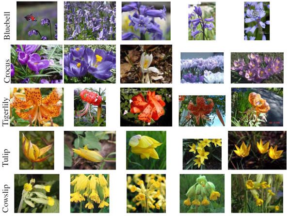
Figure 1 – A sample of the Flowers 17 Dataset. As we can see, some flowers might be indistinguishable using color or shape alone (i.e. Tulip and Cowslip have similar color distributions). Better results can be obtained by extracting both color and shape features.
If we wanted to describe these images with the intention of building an image search engine, the first descriptor I would use is color. By characterizing the color of the petals of the flower, our search engine will be able to return flowers of similar color tones.
However, just because our image search engine will return flowers of similar color, does not mean all the results will be relevant. Many flowers can have the same color but be an entirely different species.
In order to ensure more similar species of flowers are returned from our flower search engine, I would then explore describing the shape of the petals of the flower.
Now we have two descriptors — color to characterize the different color tones of the petals, and shape to describe the outline of the petals themselves.
Using these two descriptors in conjunction with one another, we would be able to build a simple image search engine for our flowers dataset.
Of course, we need to know how to index our dataset.
Right now we simply know what descriptors we will use to describe our images.
But how are we going to apply these descriptors to our entire dataset?
In order to answer that question, today we are going to explore the second step of building an image search engine: Indexing Your Dataset.
Indexing Your Dataset
Definition: Indexing is the process of quantifying your dataset by applying an image descriptor to extract features from each and every image in your dataset. Normally, these features are stored on disk for later use.
Using our flowers database example above, our goal is to simply loop over each image in our dataset, extract some features, and store these features on disk.
It’s quite a simple concept in principle, but in reality, it can become very complex, depending on the size and scale of your dataset. For comparison purposes, we would say that the Flowers 17 dataset is small. It has a total of only 1,360 images (17 categories x 80 images per category). By comparison, image search engines such as TinEye have image datasets that number in the billions.
Let’s start with the first step: instantiating your descriptor.
1. Instantiate Your Descriptor
In my How-To guide to building an image search engine, I mentioned that I liked to abstract my image descriptors as classes rather than functions.
Furthermore, I like to put relevant parameters (such as the number of bins in a histogram) in the constructor of the class.
Why do I bother doing this?
The reason for using a class (with descriptor parameters in the constructor) rather than a function is because it helps ensure that the exact same descriptor with the exact same parameters is applied to each and every image in my dataset.
This is especially useful if I ever need to write my descriptor to disk using cPickle and load it back up again farther down the line, such as when a user is performing a query.
In order to compare two images, you need to represent them in the same manner using your image descriptor. It wouldn’t make sense to extract a histogram with 32 bins from one image and then a histogram with 128 bins from another image if your intent is to compare the two for similarity.
For example, let’s take a look at the skeleton code of a generic image descriptor in Python:
|
1
2
3
4
5
6
7
8
9
10
|
class GenericDescriptor:
def __init__(self, paramA, paramB):
# store the parameters for use in the ‘describe’ method
self.paramA = paramA
self.paramB = paramB
def describe(self, image):
# describe the image using self.paramA and self.paramB
# as supplied in the constructor
pass
|
The first thing you notice is the __init__ method. Here I provide my relevant parameters for the descriptor.
Next, you see the describe method. This method takes a single parameter: the image we wish to describe.
Whenever I call the describe method, I know that the parameters stored during the constructor will be used for each and every image in my dataset. This ensures my images are described consistently with identical descriptor parameters.
While the class vs. function argument doesn’t seem like it’s a big deal right now, when you start building larger, more complex image search engines that have a large codebase, using classes helps ensure that your descriptors are consistent.
2. Serial or Parallel?
A better title for this step might be “Single-core or Multi-core?”
Inherently, extracting features from images in a dataset is a task that can be made parallel.
Depending on the size and scale of your dataset, it might make sense to utilize multi-core processing techniques to split-up the extraction of feature vectors from each image between multiple cores/processors.
However, for small datasets using computationally simple image descriptors, such as color histograms, using multi-core processing is not only overkill, it adds extra complexity to your code.
This is especially troublesome if you are just getting started working with computer vision and image search engines.
Why bother adding extra complexity? Debugging programs with multiple threads/processes is substantially harder than debugging programs with only a single thread of execution.
Unless your dataset is quite large and could greatly benefit from multi-core processing, I would stay away from splitting the indexing task up into multiple processes for the time being. It’s not worth the headache just yet. Although, in the future I will certainly have a blog post discussing best practice methods to make your indexing task parallel.
3. Writing to Disk
This step might seem a bit obvious. But if you’re going to go through all the effort to extract features from your dataset, it’s best to write your index to disk for later use.
For small datasets, using a simple Python dictionary will likely suffice. The key can be the image filename (assuming that you have unique filenames across your dataset) and the value the features extracted from that image using your image descriptor. Finally, you can dump the index to file using cPickle.
If your dataset is larger or you plan to manipulate your features further (i.e. scaling, normalization, dimensionality reduction), you might be better off using h5py to write your features to disk.
Is one method better than the other?
It honestly depends.
If you’re just starting off in computer vision and image search engines and you have a small dataset, I would use Python’s built-in dictionary type and cPickle for the time being.
If you have experience in the field and have experience with NumPy, then I would suggest giving h5py a try and then comparing it to the dictionary approach mentioned above.
For the time being, I will be using cPickle in my code examples; however, within the next few months, I’ll also start introducing h5py into my examples as well.
Summary
Today we explored how to index an image dataset. Indexing is the process of extracting features from a dataset of images and then writing the features to persistent storage, such as your hard drive.
The first step to indexing a dataset is to determine which image descriptor you are going to use. You need to ask yourself, what aspect of the images are you trying to characterize? The color distribution? The texture and tactile quality? The shape of the objects in the image?
After you have determined which descriptor you are going to use, you need to loop over your dataset and apply your descriptor to each and every image in the dataset, extracting feature vectors. This can be done either serially or parallel by utilizing multi-processing techniques.
Finally, after you have extracted features from your dataset, you need to write your index of features to file. Simple methods include using Python’s built-in dictionary type and cPickle. More advanced options include using h5py.
Next week we’ll move on to the third step in building an image search engine: determining how to compare feature vectors for similarity.
Building an Image Search Engine: Defining Your Similarity Metric (Step 3 of 4)
First, let’s have a quick review.
Two weeks ago we explored the first step of building an image search engine: Defining Your Image Descriptor. We explored three aspects of an image that can easily be described: color, texture, and shape.
From there, we moved on to Step 2: Indexing Your Dataset. Indexing is the process of quantifying our dataset by applying an image descriptor to extract features from every image in our dataset.
Indexing is also a task that can easily be made parallel — if our dataset is large, we can easily speedup the indexing process by using multiple cores/processors on our machine.
Finally, regardless if we are using serial or parallel processing, we need to write our resulting feature vectors to disk for later use.
Now, it’s time to move onto the third step of building an image search engine: Defining Your Similarity Metric
Defining Your Similarity Metric
Today we are going to perform a CURSORY review of different kinds of distance and similarity metrics that we can use to compare two feature vectors.
Note: Depending on which distance function you use, there are many, many “gotchas” you need to look out for along the way. I will be reviewing each and every one of these distance functions and providing examples on how to properly use them later on in this blog, but don’t blindly apply a distance function to feature vectors without first understanding how the feature vectors should be scaled, normalized, etc., otherwise you might get strange results.
So what’s the difference between a distance metric and a similarity metric?
In order to answer this question we first need to define some variables.
Let d be our distance function, and x, y, and z be real-valued feature vectors, then the following conditions must hold:
- Non-Negativity:
d(x, y) >= 0. This simply means that our distance must be non-negative. - Coincidence Axiom:
d(x, y) = 0if and only ifx = y. A distance of zero (meaning the vectors are identical) is only possible if the two vectors have the same value. - Symmetry:
d(x, y) = d(y, x). In order for our distance function to be considered a distance metric, the order of the parameters in the distance should not matter. Specifyingd(x, y)instead ofd(y, x)should not matter to our distance metric and both function calls should return the same value. - Triangle Inequality:
d(x, z) <= d(x, y) + d(y, z). Do you remember back to your high school trig class? All this condition states is that the sum of the lengths of any two sides must be greater than the remaining side.
If all four conditions hold, then our distance function can be considered a distance metric.
So does this mean that we should only use distance metrics and ignore other types of similarity metrics?
Of course not!
But it’s important to understand the terminology, especially when you go off building image search engines on your own.
Let’s take a look at five of the more popular distance metrics and similarity functions. I’ve included links to the function’s corresponding SciPy documentation just in case you want to play with these functions yourself.
- Euclidean: Arguably the most well known and must used distance metric. The euclidean distance is normally described as the distance between two points “as the crow flies”.
- Manhattan: Also called “Cityblock” distance. Imagine yourself in a taxicab taking turns along the city blocks until you reach your destination.
- Chebyshev: The maximum distance between points in any single dimension.
- Cosine: We won’t be using this similarity function as much until we get into the vector space model, tf-idf weighting, and high dimensional positive spaces, but the Cosine similarity function is extremely important. It is worth noting that the Cosine similarity function is not a proper distance metric — it violates both the triangle inequality and the coincidence axiom.
- Hamming: Given two (normally binary) vectors, the Hamming distance measures the number of “disagreements” between the two vectors. Two identical vectors would have zero disagreements, and thus perfect similarity.
This list is by no means exhaustive. There are an incredible amount of distance functions and similarity measures. But before we start diving into details and exploring when and where to use each distance function, I simply wanted to provide a 10,000ft overview of what goes into building an image search engine.
Now, let’s compute some distances:
|
1
2
3
4
5
6
7
8
9
|
>>> from scipy.spatial import distance as dist
>>> import numpy as np
>>> np.random.seed(42)
>>> x = np.random.rand(4)
>>> y = np.random.rand(4)
>>> x
array([ 0.37454012, 0.95071431, 0.73199394, 0.59865848])
>>> y
array([ 0.15601864, 0.15599452, 0.05808361, 0.86617615])
|
The first thing we are going to do is import the packages that we need: the distance module of SciPy and NumPy itself. From there, we need to seed the pseudo-random number generator with an explicit value. By providing an explicit value (in this case, 42), it ensures that if you were to execute this code yourself, you would have the same results as me.
Finally, we generate our “feature vectors”. These are real-valued lists of length 4, with values in the range [0, 1].
Time to compute some actual distances:
|
1
2
3
4
5
6
|
>>> dist.euclidean(x, y)
1.0977486080871359
>>> dist.cityblock(x, y)
1.9546692556997436
>>> dist.chebyshev(x, y)
0.79471978607371352
|
So what does this tell us?
Well, the Euclidean distance is smaller than the Manhattan distance. Intuitively, this makes sense. The Euclidean distance is “as the crow flies” (meaning that it can take the shortest path between two points, like an airplane flying from one airport to the other). Conversely, the Manhattan distance more closely resembles driving through the blocks of a city — we are making sharp angled turns, like driving on a piece of grid paper, thus the Manhattan distance is larger since it takes us longer to travel the distance between the two points.
Finally, the Chebyshev distance is the maximum distance between any two components in the vector. In this case, a maximum distance of 0.794 is found from |0.95071431 – 0.15599452|.
Now, let’s take a look at the Hamming distance:
|
1
2
3
4
5
6
7
8
|
>>> x = np.random.random_integers(0, high = 1, size =(4,))
>>> y = np.random.random_integers(0, high = 1, size =(4,))
>>> x
array([1, 1, 1, 0])
>>> y
array([1, 0, 1, 1])
>>> dist.hamming(x, y)
0.5
|
In the previous example we had real-valued feature vectors. Now we have binary feature vectors. The Hamming distance compares the number of mis-matches between the x and yfeature vectors. In this case it finds two mis-matches — the first being at x[1] and y[1] and the second being at x[3] and y[3].
Given that we have two mis-matches and the vectors are of length four, the ratio of mis-matches to the length of the vector is 2 / 4 = 0.5, thus our Hamming distance.
Summary
The first step in building an image search engine is to decide on an image descriptor. From there, the image descriptor can be applied to each image in the dataset and a set of features extracted. This process is called “indexing a dataset”. In order to compare two feature vectors and determine how “similar” they are, a similarity measure is required.
In this blog post we performed an cursory exploration of distance and similarity functions that can be used to measure how “similar” two feature vectors are.
Popular distance functions and similarity measures include (but are certainly not limited to): Euclidean distance, Manhattan (city block), Chebyshev, Cosine distance, and Hamming.
Not only will we explore these distance functions in further detail later on in this blog, but I will also introduce many more, including methods geared specifically to comparing histograms, such as the correlation, intersection, chi-squared, and Earth Movers Distance methods.
At this point you should have a basic idea of what it takes to build an image search engine. Start extracting features from images using simple color histograms. Then compare them using the distance functions discussed above. Note your findings.
Building an Image Search Engine: Searching and Ranking (Step 4 of 4)
We are now at the final step of building an image search engine — accepting a query image and performing an actual search.
Let’s take a second to review how we got here:
- Step 1: Defining Your Image Descriptor. Before we even consider building an image search engine, we need to consider how we are going to represent and quantify our image using only a list of numbers (i.e. a feature vector). We explored three aspects of an image that can easily be described: color, texture, and shape. We can use one of these aspects, or many of them.
- Step 2: Indexing Your Dataset. Now that we have selected a descriptor, we can apply the descriptor to extract features from each and every image in our dataset. The process of extracting features from an image dataset is called “indexing”. These features are then written to disk for later use. Indexing is also a task that is easily made parallel by utilizing multiple cores/processors on our machine.
- Step 3: Defining Your Similarity Metric. In Step 1, we defined a method to extract features from an image. Now, we need to define a method to compare our feature vectors. A distance function should accept two feature vectors and then return a value indicating how “similar” they are. Common choices for similarity functions include (but are certainly not limited to) the Euclidean, Manhattan, Cosine, and Chi-Squared distances.
Finally, we are now ready to perform our last step in building an image search engine: Searching and Ranking.
The Query
Before we can perform a search, we need a query.
The last time you went to Google, you typed in some keywords into the search box, right? The text you entered into the input form was your “query”.
Google then took your query, analyzed it, and compared it to their gigantic index of webpages, ranked them, and returned the most relevant webpages back to you.
Similarly, when we are building an image search engine, we need a query image.
Query images come in two flavors: an internal query image and an external query image.
As the name suggests, an internal query image already belongs in our index. We have already analyzed it, extracted features from it, and stored its feature vector.
The second type of query image is an external query image. This is the equivalent to typing our text keywords into Google. We have never seen this query image before and we can’t make any assumptions about it. We simply apply our image descriptor, extract features, rank the images in our index based on similarity to the query, and return the most relevant results.
You may remember that when I wrote the How-To Guide on Building Your First Image Search engine, I included support for both internal and external queries.
Why did I do that?
Let’s think back to our similarity metrics for a second and assume that we are using the Euclidean distance. The Euclidean distance has a nice property called the Coincidence Axiom, implying that the function returns a value of 0 (indicating perfect similarity) if and only if the two feature vectors are identical.
If I were to search for an image already in my index, then the Euclidean distance between the two feature vectors would be zero, implying perfect similarity. This image would then be placed at the top of my search results since it is the most relevant. This makes sense and is the intended behavior.
How strange it would be if I searched for an image already in my index and did not find it in the #1 result position. That would likely imply that there was a bug in my code somewhere or I’ve made some very poor choices in image descriptors and similarity metrics.
Overall, using an internal query image serves as a sanity check. It allows you to make sure that your image search engine is functioning as expected.
Once you can confirm that your image search engine is working properly, you can then accept external query images that are not already part of your index.
The Search
So what’s the process of actually performing a search? Checkout the outline below:
1. Accept a query image from the user
A user could be uploading an image from their desktop or from their mobile device. As image search engines become more prevalent, I suspect that most queries will come from devices such as iPhones and Droids. It’s simple and intuitive to snap a photo of a place, object, or something that interests you using your cellphone, and then have it automatically analyzed and relevant results returned.
2. Describe the query image
Now that you have a query image, you need to describe it using the exact same image descriptor(s) as you did in the indexing phase. For example, if I used a RGB color histogram with 32 bins per channel when I indexed the images in my dataset, I am going to use the same 32 bin per channel histogram when describing my query image. This ensures that I have a consistent representation of my images. After applying my image descriptor, I now have a feature vector for the query image.
3. Perform the Search
To perform the most basic method of searching, you need to loop over all the feature vectors in your index. Then, you use your similarity metric to compare the feature vectors in your index to the feature vectors from your query. Your similarity metric will tell you how “similar” the two feature vectors are. Finally, sort your results by similarity.
If you would like to see the “Performing the Search” step in action, head on over to my How-To Guide on Building Your First Image Search Engine post. On Step #3, I give you Python code that can be used to perform a search.
Looping over your entire index may be feasible for small datasets. But if you have a large image dataset, like Google or TinEye, this simply isn’t possible. You can’t compute the distance between your query features and the billions of feature vectors already present in your dataset.
For the readers that have experience in information retrieval (traditionally focused on building text search engines), we can also use tf-idf indexing and an inverted index to speedup the process. However, in order to use this method, we need to ensure our features can fit into the vector space model and are sufficiently sparse. Building an image search engine that utilizes this method is outside the scope of this post; however, I will certainly be revisiting it in the future when we start to build more complex search engines.
4. Display Your Results to the User
Now that we have a ranked list of relevant images we need to display them to the user. This can be done using a simple web interface if the user is on a desktop, or we can display the images using some sort of app if they are on a mobile device. This step is pretty trivial in the overall context of building an image search engine, but you should still give thought to the user interface and how the user will interact with your image search engine.
Summary
So there you have it, the four steps of building an image search engine, from front to back:
- Define your image descriptor.
- Index your dataset.
- Define your similarity metric.
- Perform a search, rank the images in your index in terms of relevancy to the user, and display the results to the user.
So what did you think of this series of posts? Was it informative? Did you learn anything? Or do you prefer posts that have more code examples, like Hobbits and Histograms?
Please leave a comment below, I would love to hear your thoughts.
Clever Girl: A Guide to Utilizing Color Histograms for Computer Vision and Image Search Engines
Building a Pokedex in Python: Indexing our Sprites using Shape Descriptors (Step 3 of 6)
Dia 20 de 21
Hi,
So I’ve been talking a lot about image descriptors and indexing lately.
And you may be wondering, what are some good datasets that I can use to practice extracting features from?
Well, here is a list of the top 5 datasets to practice with:
- Amsterdam Library of Object Images
- CALTECH-101
- Flowers 17
- Flickr Material Database
- CALTECH-UCSD Birds 200
I built my first image search engine using the Amsterdam Library of Object Images.
First, I took roughly 20 categories of images from the original dataset and then wrote code to extract flattened RGB color histograms from them. Then, I compared my color histograms using the euclidean distance for relevancy.
I suggest you go ahead and give that a shot.
When you are done, send me an email with your code. I would be happy to discuss it with you and give you some pointers.
Cheers,
Adrian Rosebrock
Chief PyImageSearcher
Dia 21 de 21
Hi,
Congrats! You’ve made it to the end of my crash course!
Take a second and congratulate yourself. You’ve learned a lot. Here’s a quick recap:
- You built your first image search engine using color histograms.
- You learned my exclusive tip on how to become awesome at computer vision: creating and building your own projects. It’s definitely not easy. And it requires a bit of work — but it’s by far the best way to learn computer vision.
- Let’s not forget about all the libraries you learned about, including OpenCV, SimpleCV.
- Avoid PIL, it’s not Pythonic and you don’t have as much control as you would with OpenCV and SimpleCV.
- You uncovered the 4 steps of building ANY image search engine: (1) defining your image descriptor, (2) indexing your dataset, (3) defining your similarity metric, and (4) search and ranking.
- Need a simple (yet effective) image descriptor? Start with color histograms.
- And if you need to describe the shape of an object? You can use Hu Moments, which are built into OpenCV.
- To find the most dominant colors in an image, cluster the pixel intensities using k-means.
- And finally, I showed you the 5 best image datasets to practice extracting features from.
Now, you may be wondering: “Where do I go from here?”